OpenADMET PXR Blind Challenge · 2026-04-01 → 07-01
Predicting PXR activation (pEC50) for 513 blinded compounds
Model report for OpenADMET PXR Challenge Track 1 (Activity) — N283T, final rank 4 of 95.
0. TL;DR
- Finished 4th of 95 (Tier 1) on the OpenADMET PXR Challenge Track 1 (Activity), predicting PXR induction (pEC50) from SMILES alone. MAE was 0.4059 on the interim leaderboard (AS1 + AS2) and 0.4113 on the final Phase 2 set (AS2).
- What decided it was multi-fidelity transfer learning (after Buterez et al. 2024). The challenge ships a cheap, single-concentration
log2fcreadout as auxiliary data, measured on 10,875 compounds against only 4,140 pEC50 labels — and a model's predicted log2fc turned out to be the single strongest feature. - Around that signal sits a nine-member Caruana ensemble. The members fall into three families — tabular core, frozen embed, and Boltz trunk — and every one of them uses TabPFN as its readout head.
- Downstream of the ensemble, the only thing that clearly helped was a single affine calibration. The late Phase 1 tail gates and the whole of Phase 2 mostly added noise or made things worse. Knowing when to stop was, in hindsight, one of the better calls.
1. The challenge
This is the Track 1 (Activity) model report for the OpenADMET PXR Induction Challenge. For the challenge background, biology, rules, and timeline, see the official pages:
This report focuses on the modeling approach and results. Exploratory data analysis and a full description of the challenge are out of scope and omitted here.
The task at a glance is in Table 1.
| Item | Value | Notes |
|---|---|---|
| Target | pEC50 | higher is a stronger PXR inducer |
| Metric | MAE | regression task |
| Training set | 4,140 | labeled compounds |
| Analog Set 1 | 253 | unblinded at the start of Phase 2 |
| Analog Set 2 | 260 | blinded throughout |
| Test total | 513 | AS1 + AS2 |
2. Results
Scores came out at three main points. The live leaderboard moved with every submission, so these three are the only standings that hold still afterwards.
Phase 1 final AS1 (253)live LBrank 8
Final score on the live leaderboard
Interim AS1 + AS2 (513)one-off LBrank 4 / 338
Same model as Phase 1 final
Phase 2 AS2 (260)no LBrank 4 / 95
Final standing — the AS1 labels were public once Phase 1 closed
MAE is the only ranked metric; the ranks for the others are our own count from the LB values.
The full final leaderboard is viewable on the challenge's Hugging Face Space (Leaderboard tab). Organizers' write-ups: Phase 1 results and the post-challenge wrap-up.
3. Strategy
The strategy was built on Buterez et al.'s paper on multi-fidelity transfer learning. In hindsight, getting to that paper was one of the biggest reasons the result landed where it did.
The auxiliary data
At first we built features and models from the Train pEC50 labels alone. But there are only 4,140 pEC50 labels, and accuracy plateaued almost immediately. The challenge data also ships a single-concentration reporter assay as auxiliary data (log2 fold-change, or log2fc, at 8.25 µM and 33 µM), and it covers far more compounds. We knew that auxiliary signal was there; we did not know how to use it well. Naive ideas such as converting it into pseudo pEC50 labels only lowered accuracy.
- Train / Test / AUX data — the three distributed sets, each with a different set of columns filled in (Table 2)
- Test is SMILES only — it carries no measured values, so no log2fc is available for Test either
- log2fc is measured at two concentrations, so there are two readings per compound
| Dataset | Compounds | SMILES | pEC50 | Emax | counter assay | log2fc 8.25 µM | log2fc 33 µM |
|---|---|---|---|---|---|---|---|
| Train | 4,140 | ✓ | ✓ | ✓ | 2,860 | 2,374 | 2,321 |
| Test | 513 | ✓ | ✗ | ✗ | ✗ | ✗ | ✗ |
| AUX data | 10,875 | ✓ | ✗ | ✗ | 2,359 | 10,752 | 9,527 |
Finding Buterez et al.
To break the plateau, we had Claude Code draft a research prompt that laid the situation out as it stood (scarce pEC50, an abundant auxiliary assay, pseudo-labeling that did not work), then asked for ways to exploit the auxiliary signal. Running that prompt through ChatGPT Deep Research surfaced Buterez et al.
What the paper compares
The paper is about the multi-fidelity situation: the tiers of a drug-screening cascade.
The paper asks how to put the cheap side to work predicting the expensive side. It compares six ways of doing it.
- 1Add the raw LF labels as features10
- 2Add the labels an LF model predicts3
- 3Hybrid — measured for training, predicted for inference2
- 4Add the LF model's embedding10
- 5Pretrain on LF, then fine-tune as usual0
- 6Pretrain on LF, fine-tune the readout only26
The number on the right is how many of the 51 cases that strategy won.
The paper concludes that adding the raw labels alone cuts MAE by 10 to 40%, and that embeddings beat that by up to a further 10%.
Adapting it
This is where our case starts. The challenge data dropped straight into the setting the paper assumes (Table 3).
| Fidelity | What it maps to here | Count |
|---|---|---|
| high-fidelity | Train pEC50 | 4,140 labels |
| low-fidelity | single-concentration log2fc | 10,875 compounds |
It differed from the paper in two main ways.
- The raw labels are unusable — Test has no measurements, so 1 and 3 were off the table from the start
- Far less LF data — the paper had over a million measurements; we had 10,875 compounds
Of what was left, we took 2 and 4.
- 2Add the predictions
log2fc_8p25_pred/log2fc_33_predas features - 4Hand over the frozen embedding of an encoder pretrained on log2fc
On top of that we put TabPFN downstream, which the paper never considers. Table 4 compares downstream models with the encoder held fixed at the same ChemProp (D-MPNN).
| Downstream | OOF MAE | Spearman |
|---|---|---|
| 4's embedding, read by TabPFN | 0.437 | 0.807 |
| 6train an adaptive readout (the paper's pick) | 0.482 | 0.758 |
| 5fine-tune directly, no freezing | 0.507 | 0.755 |
The more we froze and the simpler we kept the downstream model, the better it got. The framework is the paper's; only the downstream part is swapped out.
Predicted log2fc: the strongest feature
This is what strategy 2 looked like in practice. We trained a ChemProp model to predict the single-concentration log2fc and added its two predicted columns (8.25 µM and 33 µM) to the features. This report calls them pred log2fc. How the predictor is built is covered below in the ChemProp member description.
The bottom row of Figure 1 is pred log2fc. It tracks pEC50 more closely than the observed row above it (r 0.75 / 0.80 vs 0.72 / 0.50), and the observed values only exist where the assay was run. Swapping in the prediction fills the coverage gap and smooths the signal at the same time.
Set beside the other features in Figure 2, the two pred log2fc columns still lead. The descriptors are all weak on their own; inside the model they work as context filling in around pred log2fc.
Accuracy is not the only thing it buys. pred log2fc is computed from SMILES, so it exists for Test as well, which carries no measured labels at all. The predicted form is therefore the only way an assay-derived signal reaches the compounds we are scored on.
How far does pred log2fc alone get? post-challenge
To size the signal, we fit a few deliberately simple models on the Train pEC50 and scored them on the now-unblinded Test, AS1 + AS2 (Table 5). The comparison point is an untuned LightGBM on the full RDKit descriptor set.
| Feature | Model | Dims | MAE | Spearman |
|---|---|---|---|---|
| pred 8.25 µM | linear | 1 | 0.609 | 0.782 |
| pred 33 µM | linear | 1 | 0.571 | 0.746 |
| pred log2fc (both) | linear | 2 | 0.572 | 0.725 |
| Boltz-2 affinity | linear | 1 | 0.747 | 0.602 |
| RDKit | LightGBM (untuned) | 217 | 0.570 | 0.677 |
| Phase 1 submission | ensemble | ~2,100 | 0.406 | 0.834 |
scripts/ablation_baselines.py). The last row is the Phase 1 submission, put there as a yardstick.A single pred log2fc column already reaches MAE 0.57 to 0.61, and two columns through a plain linear fit match the untuned 217-dimension LightGBM (0.570). On rank correlation they are ahead (Spearman 0.72 to 0.78 vs 0.68). All of them clearly beat the Boltz-2 affinity score (0.75). Predicting a single assay-derived signal does the work of one whole generic descriptor model.
4. The ensemble
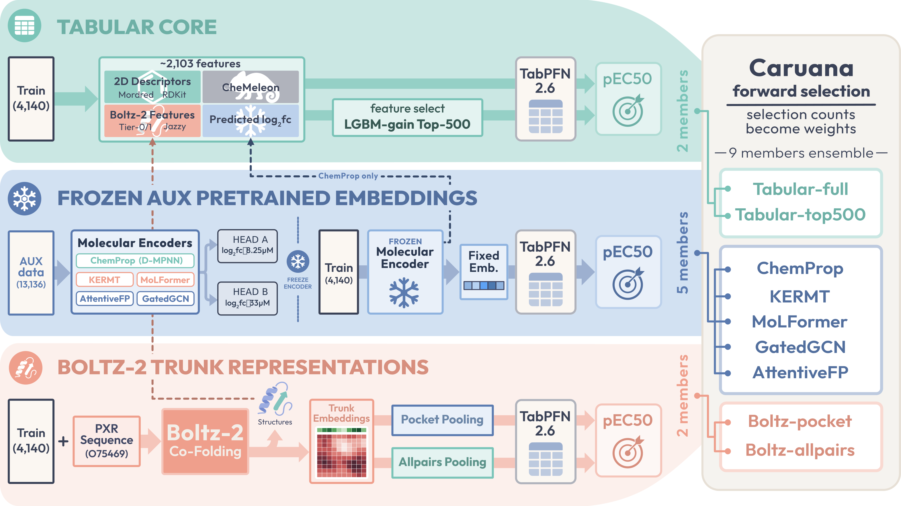
The final system is an ensemble of nine members (Figure 3). The only thing that varies between them is how the features are built, and that splits three ways.
- tabular core — the 2,103 dimensions of descriptors and pred log2fc, passed through unchanged
- frozen embed — an encoder pretrained on log2fc, frozen; its embedding goes in instead
- Boltz trunk — the internal representation from Boltz-2
- the only family with no log2fc in it
The readout head is TabPFN for every member; all that differs is what sits in front of it.
The nine members, with the aliases used from here on, are in Table 6.
| Alias | Encoder / features | Family | Strategy | OOF MAE | Weight |
|---|
The CV split is a UMAP cluster split (Morgan FP + UMAP → KMeans). Of the ones we tried it tracked the public LB most closely; that is the whole case for it, not that it is a better split. To combine the members we used Caruana forward selection (Caruana et al., ICML 2004). What we submitted was not this ensemble itself but its output with a post-hoc calibration and gate layered on top (6. Calibration).
How independent are the members? post-challenge
Not very. All 36 pairs land between 0.81 and 0.98, mean 0.88 (Figure 4). Members sharing the same log2fc running high is no surprise, but even the Boltz trunk members, which carry no log2fc at all, sit at 0.81 to 0.88 against the rest. What that says is that there is no cue stronger than log2fc, and that there was not much information to go around in the first place.
This is correlation between test predictions, though, not the OOF correlation Caruana used to set the weights. Recomputed out-of-fold it becomes 0.90 to 0.99, mean 0.93, and the small gap where Boltz sat lower disappears too.
The ensemble still earns its place, not because it blends independent views but because it works as a buffer. Drop the low-weight members and one family's share climbs to 0.94, while the public LB gets 0.006 worse. What the small members do is stop a strong but highly correlated member (top500 above all) from taking over the prediction. That is also why progress stalled. Round after round, new models either got rejected as too correlated or made things worse when we forced them in, so we moved our focus to calibration and the gate.
5. The members
This section opens up the three families one at a time, using the aliases. Standalone OOF MAE and Caruana weights are in the table in Section 4.
5.1 Tabular core (tabular-full, tabular-top500)
The two highest-weighted members share a single feature stack: a roughly 2,103-dimension tabular matrix built by concatenating complementary blocks.
| Block | Dims | What it is |
|---|---|---|
| Mordred | 1,515 | 2D molecular descriptors |
| CheMeleon | 300 | ChemProp-MPNN foundation fingerprint |
| RDKit | 217 | standard RDKit descriptors |
| Boltz-2 tier-1 | 44 | pocket-level pLDDT / PAE / PDE re-aggregations |
| Boltz-2 tier-0 | 19 | pose, confidence, and affinity scalars |
| pose-Jazzy | 6 | H-bond / hydration on the Boltz pose |
| pred log2fc | 2 | the pred log2fc columns from Strategy (8.25 and 33 µM) |
CheMeleon
CheMeleon is not strong on its own (a TabPFN reading CheMeleon alone scores about 0.512 MAE). Added to the stack it clearly helped anyway: the same tabular core improved from 0.443 to 0.421.
Those 300 dimensions are an implementation mistake. The plan was to use CheMeleon's own 2,048 dimensions, but the Claude Code run that built the features saved the pretrained 2,048-dimension vector after pushing it through an untrained 2048→300 projection.
We checked the 2,048-dimension version after the challenge: getting it right would not have improved the submission. On its own, OOF improves from 0.5118 to 0.4983 while Test moves the wrong way, 0.5099 to 0.5132; mixed into the full stack it is worse there too. See PR #233 for details.
Boltz-2 features
Boltz-2 contributes three blocks, 69 dimensions in all (Table 8).
| Block | Dims | What it is |
|---|---|---|
| tier-0 | 19 | Boltz's own scalar outputs: affinity, binding probability, and confidence |
| tier-1 | 44 | per-token confidence tensors (pLDDT / PAE / PDE) re-aggregated into pocket- and ligand-level statistics |
| pose-Jazzy | 6 | ligand H-bond and hydration free energies computed on the Boltz pose (Jazzy) |
top-500 selection
TabPFN is sensitive to how many columns it gets, so handing it all 2,103 is not necessarily best. tabular-top500 keeps only the top 500 columns by per-fold LightGBM gain (tabular-full is the one that passes everything straight through). Sweep K and the curve bottoms out between 500 and 600 (Figure 5); MAE was flat across that range, so we settled on 500, where Spearman was best.
Using LightGBM for the selection also buys a little interpretability, because its gain says what the model leaned on. About three quarters of the gain sits on the two pred log2fc columns, and the rest is spread thinly across Mordred and CheMeleon (Figure 6). What the selector really does is keep the two pred log2fc columns and fill out the space with descriptors.
Zoom in on individual features and the same story gets sharper (Table 9). The two pred log2fc columns are first and second by a wide margin (52% and 22% of the gain),
and after them no single feature reaches even 0.4%. The tail is a mix of CheMeleon dimensions and readable descriptors like
SLogP, qed, and the pose-Jazzy hydration terms.
| Feature | Family | Gain share |
|---|---|---|
| log2fc_8p25_pred | pred log2fc | 51.6% |
| log2fc_33_pred | pred log2fc | 22.1% |
| chemeleon_067 | CheMeleon | 0.30% |
| chemeleon_006 | CheMeleon | 0.23% |
| chemeleon_175 | CheMeleon | 0.20% |
| chemeleon_131 | CheMeleon | 0.19% |
| SLogP | Mordred | 0.18% |
| sa | pose-Jazzy | 0.16% |
| chemeleon_002 | CheMeleon | 0.16% |
| qed | RDKit | 0.13% |
| dgtot | pose-Jazzy | 0.12% |
| chemeleon_240 | CheMeleon | 0.12% |
Why both?
On their own the two perform almost identically (OOF 0.396 against 0.397). The problem is that the benefit of the selection looks confined to OOF. Compared under matched conditions after the challenge, top500 beats full out-of-fold, 0.3968 against 0.4056, but the order flips on Test, 0.4327 against 0.4281 (PR #233). The natural reading is that the per-fold selection is itself what flatters the OOF number.
We did not understand that at the time, but keeping both and letting Caruana split the weight almost evenly (0.309 for top500, 0.288 for full) turned out to be insurance against exactly this gap. In fact, a swap that leaned harder on top500 (id56) looked best out-of-fold yet made the public LB worse, 0.4071 → 0.4135.
Re-optimizing the weights against the released AS2 labels puts numbers on the same point (issue #222, Table 10). The 0.31 we actually used sits close to the AS2-optimal 0.33, whereas optimizing against OOF inflates it to 0.84 and degrades AS2 to 0.422.
| Weighting | top500 weight | AS2 MAE |
|---|---|---|
| Our weights (as used) | 0.31 | 0.405 |
| Zero the top500 weight | 0.00 | 0.402 |
| Optimized on AS2 (oracle) | 0.33 | 0.399 |
| Optimized on OOF | 0.84 | 0.422 |
5.2 Frozen embeddings (ChemProp, KERMT, MoLFormer, GatedGCN, AttentiveFP)
These five are strategy 4 rolled out across different backbones. Pretrain an encoder on log2fc, freeze it, and hand the fixed-length vector it produces to TabPFN (Adapting it). Not fine-tuning the encoder on pEC50 was the better choice, as Table 4 in that same subsection shows.
ChemProp
ChemProp is the prototype for this recipe and the strongest member of the embedding family. It also does double duty. The same log2fc-predicting ChemProp produces the tabular core's pred log2fc columns, and the 256-dimension frozen embedding taken from that D-MPNN is this member. The same signal goes in two ways, once as a sharp prediction and once as a spread-out representation.
The pretraining is multi-task, with one regression head per concentration. It runs over all 13,136 compounds, with missing targets masked. Hyperparameters come from an Optuna search, but the objective is the downstream pEC50 OOF MAE rather than the log2fc loss.
What sharpened pred log2fc was seed averaging: pretrain with several seeds and average the predictions. Going from 5 to 10 seeds improved the downstream result (top500 OOF MAE 0.399 to 0.397), and the gain tapered off at 15 seeds, so we stopped there.
The OOF numbers in Table 4 oversold the frozen recipe's margin. ChemProp trained directly on pEC50 is weak out-of-fold at about 0.53, yet on Test it reaches about 0.48, much closer to the frozen embedding member's 0.44. The winner does not change, but OOF exaggerated the size of the gap.
Foundation encoders: KERMT & MoLFormer
The same recipe applied to larger pretrained backbones.
- KERMT — graph transformer
- continued pretraining on log2fc for a 3,200-dimension embedding; second in the embedding family (0.448 / weight 0.111)
- MoLFormer — SMILES transformer (DeepChem MoLFormer-c3)
- LoRA pretraining on log2fc, then the frozen 768-dimension [CLS] vector (0.475 / weight 0.040)
Other backbones went through the same recipe and never made the cut. ChemBERTa sat around 0.53 out-of-fold, and UniMol-v2 got to about 0.484, close to the members that stayed, but neither passed Caruana's add-value test. Fine-tuning MoLFormer-XL straight to pEC50 was also weak at 0.529, the same outcome as with ChemProp.
Extra GNNs: GatedGCN & AttentiveFP
The same frozen recipe on two more GNN backbones. Several were tried and these two simply came out best; there is nothing meaningful about the architectures themselves. Alone they are weak (0.474, 0.484) and their weights are tiny (0.017, 0.002).
They stay because they are a buffer. Take away about 0.02 of weight and the core picks up about 0.1 of it, and as Section 4 shows, the LB gets worse. A small weight does not mean a member is safe to drop.
5.3 Boltz trunk (Boltz-pocket, Boltz-allpairs)
These two use Boltz-2's trunk, its internal learned representation, and never touch the predicted structure.
The original plan was to co-fold PXR (UniProt O75469, 434 residues) with each ligand and read activity off the pose or the affinity score. That did not pan out; it survives only as weak columns inside the tabular core (Table 7). So we looked at using it as a representation instead.
We pool the trunk's s and z into 1,024 dimensions per compound
and hand that to TabPFN (Figure 7). The two members differ only in which residues feed z.
- Boltz-pocket — a fixed 13-residue core pocket crossed with the ligand atoms
- Boltz-allpairs — all 434 residues crossed with the ligand atoms
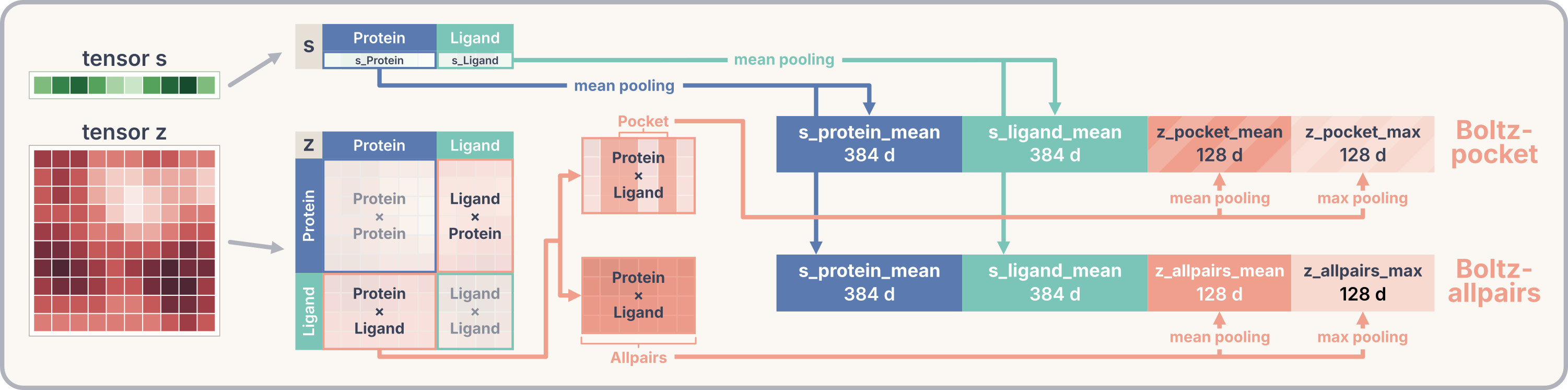
s and z come down to 1,024 dimensions. The s blocks (768 dimensions) are the same for both members.
We tried more than 20 poolings, and what carried the signal was z, the pair representation (Figure 8).
The 128-dimension z alone reaches 0.490, close on the heels of 0.486 for the full vector, while s only gets to 0.507 with 768 dimensions.
The relationship between residues and ligand atoms matters more than the shape of the ligand by itself,
which fits the fact that Boltz-2's own affinity module is designed around pairs.
By contrast, which residues you pool over barely matters: pocket and allpairs land within 0.001 MAE of each other, both about 0.486.
The trunk dimensions have no interpretable names, so a non-linear readout helps. On the same vector, TabPFN (0.486) beat LightGBM and an MLP (0.512, 0.538).
Step back, and these two are the only members of the nine that carry no log2fc. Reaching about 0.486 without the signal every other member rests on is more than we would have guessed, the more so next to the direct MoLFormer-XL fine-tune, which stalled at 0.529.
For this target at least, Boltz-2 was worth more read as a learned representation than used for its predicted structure or affinity. Pulling out only the trunk, without generating structures or running long diffusion, is cheap enough to apply to large compound sets. There may be something in using it as a protein-aware feature extractor rather than a tool for producing poses. This is one target, PXR, so it is too early to claim it generalizes.
6. Calibration
This started as a diagnosis. Spearman, Kendall and R² were all near the top, and only MAE and RAE were bad. The ordering of which compounds are potent was right; the scale and center of the predicted pEC50 were off. So instead of adding another member, we corrected the output after the fact with an affine fit.
- Build the weights — a classifier on Morgan fingerprints separates Train from Test, and the
density ratio P(test|x) / (1 − P(test|x)) becomes a per-compound weight
- Clipping to [1/3, 3] is essential; too strong a classifier lets a handful of test-like compounds pull the fit
- Fit the line — with those weights, fit an affine map from the 4,140 OOF predictions to the true labels (validated under 5-fold nested CV)
- The slope is positive, so the ordering survives untouched and only the scale and the center move
- Apply it to Test — the same affine map goes straight onto the test predictions
- The only thing it uses is the structures of the test compounds; no label is ever seen
How much did it buy? post-challenge
In the submission history the calibration effect and the member improvements are tangled together. So we regenerated raw and calibrated predictions at the final ensemble weights from one single run (unblinded Test, 513 compounds, Table 11).
| Metric | Ensemble only | + calibration |
|---|
MAE goes 0.4209 → 0.4077 and bias −0.056 → +0.002. Spearman does not move a digit from 0.8370. That is what a monotone transform has to do, but it also confirms the fix fits the diagnosis: the ranking was already right. AS1 goes 0.4191 → 0.4076 and AS2 0.4226 → 0.4078, so both splits move the same way.
It does not help everywhere, though. The gain sits mostly on the potent side (Figure 9).
The predictions really do spread back out. Against a true standard deviation of 0.996, the raw predictions sit at 0.703 and the calibrated ones at 0.767. The habit of calling potent compounds too weak and weak compounds too potent is pulled back by as much as an affine fit can manage.
7. Gates
From here on it is competition craft, not research. Swap a member, add a gate, submit, keep whatever lowered the error. All of it was done watching the public LB. Figure 10 is the last 11 submissions of Phase 1.
The final submission, id55, takes the calibrated ensemble (id51) and nudges only the compounds that look like potent-46 toward the top500 member.
id55 = id51 + 0.35 * soft_gate(nn_tanimoto_to_potent46 >= 0.40)
* (seed10_top500 - ens_caruana_bag20)- potent-46 — Test is an analog set built around strong inducers
- As a sample of that band we took the 46 training compounds with pEC50 ≥ 6 and selectivity of at least 1.5 against the counter assay
- gate — for each test compound, measure the Morgan nearest-neighbor Tanimoto to potent-46 and open only for the close ones
- 0 below 0.40, 1 at 0.55 and above, linear in between
- A hard threshold makes the predictions jump at the boundary
- How far to nudge — add 0.35 of the difference between the top500 member and the plain blend
- It adds rather than replaces, so a compound whose gate is closed stays exactly at id51
We kept trying after id55 (an Optuna-tuned member swap, id56; a looser potent gate, id57; rank versions of the gate, id58 and id59), and none of them beat it, so we resubmitted the identical file as id60 and closed out Phase 1. That is our final entry.
Nothing we added fixed the tail. The pEC50 ≥ 6 band comes out systematically low, with a bias of about −0.8 over that interval. It shrinks toward the mean by nearly a full log unit, and a global calibration does not reach that far. We tried lifting the band outright, and descriptor gates (log2fc, ring count, family gap), but on the public LB none of them separated from noise. It is the one problem Phase 1 left standing.
8. Phase 1 → Phase 2
We ended Phase 1 by giving up on chasing the LB and resubmitting the anchor unchanged. It looked timid at the time, but the blinded final scoring put us 4th of 95. Not overfitting the public LB was one of the better calls of Phase 1.
Phase 2 ran fully blind, with no public LB to steer by. Checked against the answer key, every change we made moved the predictions the wrong way (Figure 11).
Phase 2 came down to three moves.
- Retraining on the AS1 labels — we added the released AS1 to the training data,
retrained top500, and blended its predictions into the anchor at 0.45.
- Adding AS1 did not improve AS2 for most members, so the blend imported error and nothing else
- A high-activity gate — a pairrank ranking model built from external ChEMBL and public PXR activity data,
following the design of Boltz-2's affinity head, which itself trains on pairs.
- Detection was good, AUC around 0.88
- Knowing which compounds to move says nothing about how far to move them
- Getting the magnitude wrong cost more than the ranking gained
- Leaving the low-activity side alone — we judged that getting it wrong there would be expensive
- It turned out to be the right call
That does not mean we should simply have left everything alone. The candidate we did not submit,
id55shape_t10top500_t40_soft_g35, reaches 0.4056 on AS2,
under the winning 0.4061. It moved too many values and failed our own preflight check, so we benched it.
Line the three up: id60, which moves nothing, is 0.4075; id55shape, which moves a lot, is 0.4056;
id63, in between, is 0.4123. The worst was the half-measure.
With no LB, though, there was no way at submission time to tell which bet was the right one.
That is what makes a blind competition hard.
In the full post-competition answer check (issue #222), an anchor-residual stacker built without ever looking at the LB lands around 0.405 over the whole Test, ahead of the importance calibration ensemble (0.407) and of everything we submitted in Phase 2. Past a certain point, the machinery we added was costing more than it bought.
9. Conclusion
On the task of predicting pEC50 from SMILES, we finished 4th of 95 teams. Three things worked technically. The fourth was not chasing any of it further.
- Transfer learning — make up for a small Train set with abundant log2fc
- pred log2fc, which exists for every compound, beats the raw labels
- The embedding of a frozen encoder, not a direct fine-tune
- TabPFN as readout — however differently the features are built,
all nine members are read out by TabPFN
- Fixing the readout let us compare representations against each other directly
- Calibration — correcting the output afterwards did more than adding members
- The correction is fit on OOF predictions against the true labels
- Test enters the weighting through structure alone, never through labels
- Knowing when to stop — the decision of whether to move at all
- Not moving was the right call in Phase 1
- Moving backfired in Phase 2
On a personal note, this was my first competition, and 4th of 95 is better than I expected going in. Two things stick with me. One is how heavily I leaned on AI coding agents and ChatGPT throughout, for literature search, for code, and as a sounding board, and how much I got out of that workflow; I want to write about it properly in a separate post. The other is that all of this ran on a single home gaming PC, and that I did it alone. Reaching Tier 1 out of 95 teams from that setup surprised me, and I am a little proud of it.
Finally, thanks to the OpenADMET team for running the PXR Induction Challenge. The task was well designed and genuinely worth working on, and the guidance and support were thoughtful from start to finish. Releasing the data and the unblinded labels afterwards is what made the post-hoc checks and the answer-checking in this report possible. Thank you.
Reproducibility and links
- This report in Markdown: MODEL_REPORT.md
- Talk slides (42-slide HTML deck, in Japanese): slide deck
- Working repository (code, feature pipeline, day-by-day logs): N283T/pxr-iduction-challenge
- Phase 1 research log: issue #100
- Phase 2 research log: issue #208
- Post-competition AS2 answer-check log: issue #222
- Challenge page: openadmet/pxr-challenge
- Data: openadmet/pxr-challenge-train-test
- Licences for the bundled libraries and fonts: report / deck